In order to preserve the academic and historical record, this deleted article is published under Fair Use. All editorial comments are marked with a light gray background.
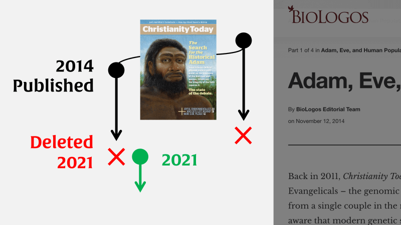
The article was first published by the BioLogos Foundation in 2014.
In 2017, this article was found to have several conclusion-altering scientific errors. January 2020, BioLogos briefly acknolwedged errors in this article. However, they declined our request to transparently correct the scientific errors here.
Instead, in June 2021, BioLogos deleted the article. They posted a new article at a different URL with different authorship. The new aricle is a substantially revised version of this deleted article, back-dated to November 12, 2014. The conclusions of the new article are substatially reivised, but the note claimed they were “unchanged.”
Insertions and deletions made to the original text in the revised article are marked.
Back in 2011, Christianity Today ran a cover article on what was fast becoming a hot-button issue for Evangelicals – the genomic science that indicates humans descend from a large population, rather than from a single couple in the relatively recent past. Since 2011 Evangelicals have become increasingly aware that modern genetic studies of humans support this conclusion; however, there remains a great deal of confusion about exactly how this genetic evidence works, and, not surprisingly, suspicion about its accuracy. In this article, we will explore several lines of genetic evidence that shed light on our species’ past in an attempt to rectify these misunderstandings.
Defining the Issues
Part of the challenge this subject generates for Evangelicals is due to confusion over exactly what the science can and cannot say about human origins in general, or the historicity of Adam and Eve in particular. Briefly stated, genetics is well suited to addressing scientific questions such as whether humans share ancestry with other forms of life, and what our population structure looked like as we separated from our evolutionary relatives. And what we see in the genetics of our species is unremarkable for a relatively large-bodied mammal – we do indeed share common ancestry with other species, and we descend from a large population that has never numbered below about 10,000 individuals throughout our evolutionary historyin the thousands as far back as we can see. Scientifically speaking, these issues are straightforward and uncontroversial.
In addition to these scientific questions, however, Evangelicals are also strongly interested in the question of Adam and Eve’s historicity: were they a literal couple that lived about 6,000 – 10,000 years ago? Unfortunately, genomic science is not at all equipped to address this question – it simply does not have the ability to establish (or rule out, for that matter) the historicity of any particular individual in the ancient past.
For many Evangelicals (or for that matter
atheists), the idea that we are the products of evolution and became human as a large population over time is on its face contradictory to the idea that Adam and Eve may have been historical individuals. The reason, of course, is not a scientific one, but rather an interpretation that the Genesis narratives preclude understanding Adam and Eve as anything other than the first humans, directly created by God without shared ancestry, who are the sole genetic progenitors of the entire human race. This is, of course, a very common evangelical interpretation of Genesis, but it is
not the only one – several
other options are available that attempt to respect both Scripture and science. After all, Genesis has long been noted to imply that Adam and Eve’s family is part of a larger unrelated population (for example Cain worries about being killed for his sin, leaves to build a city elsewhere, and takes a wife in the process). The fact that Genesis presents these facets of the story without comment or clarification also shows us, in my opinion, that the narrative is simply not concerned with telling the story of our genetic origins but rather is focused on theological concernsconcerned with more than telling the story of our genetic origins.
So, the decision to equate the historicity of Adam and Eve with the expectation that humans descend uniquely from an ancestral couple is a hermeneutical one, not a scientific one. As such, the historicity question needs to be addressed hermeneutically, not scientifically – it simply lies outside the purview of what genetics can tell us.
Evolution as a population level phenomenon
Aside from the hermeneutical issues surrounding human evolution and population genetics (which are confusing enough for many of us), there are the scientific issues – which, for many Evangelicals, are similarly fraught with misunderstanding. One of the main misconceptions is failing to understand that evolution is a population-level phenomenon: species typically form slowly, as populations, due to the accumulation of numerous slight genetic differences that shift the average characteristics of a population over time. All that is required to start this process is to have some sort of genetic barrier between two populations – perhaps a geographic barrier to start. Once two populations of the same species are reproductively isolated, genetic changes in the one population are not shared with the other – and vice versa. Over many, many generations enough changes may accumulate in the two populations that their average characteristics are different enough such that they would no longer recognize each other as members of the same species. At this point, even if the two populations were brought into contact again, these differences (perhaps behavioral or physical) would keep the genetic barrier in place by reducing or preventing interbreeding, and thus prevent the two groups from collapsing back into one large population.
If, on the other hand, one is used to thinking that species form when they are founded by a pair that has undergone a marked genetic change compared to their source population, one is more likely to think that it would have been possible for humans to get their start in such fashion. These sorts of misunderstandings are common among non-scientists, and Evangelicals are not immune to them. For example, even among Christians who accept that we share ancestry with other life, I frequently get askedpeople frequently ask what was “the mutation” was that “made us human”.? Sometimes, folkspeople wonder how such a dramatic mutation could have occurred in two individuals at the same time to provide a male and female member of the same (brand new!) species – and speculate that God must have directed it to occur to form Adam and Eve. Their understanding of human speciation is that it was sudden, involved only one couple, and required dramatic genetic change. In reality, speciation is almost always precisely the opposite: it’s slow, takes place in a population, and requires the accumulation of many discrete genetic differences, none of which are particularly dramatic. Next, we’ll begin to explore how a population can accumulate genetic changes, and perhaps shift its average characteristics over time – beginning with how genetic diversity arises in the first place.
A Primer on Population Genetics
Evolution as gradual change at the population level
One of the most common misunderstandings about evolution is failing to appreciate that evolution happens to populations, not individuals. But, you might interject, populations are made up of individuals – so how does that work? The answer is that yes, genetic variation enters a population through mutations in individuals – but that only when such variation accumulates within a population and shifts its average characteristics do we observe its effects.
Perhaps an analogy will help here –
one that I have used before, that of language change over time. Languages are like populations – they have a large number of individuals who speak it. While each individual has their own particular quirks (favorite phrases, word preferences, and perhaps even chronic spelling mistakes) any one person cannot, on the whole, cause significant change to their language within their lifetimes. Additionally, any person who does change radically from their language group will effectively be placing themselves outside it – if their changes are large enough to hinder their intelligibility to others. So, language evolution is not an individual affair. Yet languages do change over time, and individuals do contribute to that change. Someone might invent a new word that catches on, for example. Others might be part of the “catching on” – hearing a new word, or new phrase, and repeating it to others. Over time (perhaps generations) a language will slowly adopt new words, new spellings, and new rules of grammar (such as
split infinitives in English – to boldly split what no man has split before – but I digress). Yet, such adoptions are gradual. They enter the language as rarities, slowly become more common, and eventually become the “normal” way of doing things (much to the chagrin of English teachers). Thankfully, such changes typically take longer than one generation, sparing those of us who cringe at the novelties of our day. If the English words “there, their and they’re” ever officially collapse into one word determined solely by context or the use of apostrophes to form plurals becomes standard, I’m thankful I won’t be here to see it.
Just as a language has many speakers, a species has many members. They must be genetically compatible – i.e. speak the same language – but they are not all genetically identical – they have their own particular variation within an acceptable range to be in the group. In other words, though populations are a unit (they interbreed) they have genetic variation.
In the terminology of genetics we can understand this in terms of genes and alleles. While all members of the population have the same genes, they do not all have exactly the same version of any given gene. Different versions of a gene are called alleles, and they arise through mutations – that is, copying errors when chromosomes are replicated. For humans, we may have up to two different alleles for any gene – the allele we inherit from our mother, and the allele we inherit from our father. If we have two different alleles, we are said to be heterozygous for that particular gene. If we have two identical alleles for a gene, we are homozygous for that gene. While any individual can have up to only two alleles, populations as a whole can have hundreds or even thousands of alleles.
In any given generation, the vast majority of the alleles present in a population were inherited from the previous generation – just like a language group learning from their parents, and picking up the language as a whole, but also some of their particular linguistic quirks. Each generation also can contribute its own novelty to the population in the form of new alleles arising through mutation – just like teenagers coming up with new words or phrases. These new alleles, are rare of course – they are only held by one individual at the beginning. Over many, many generations, however, such new alleles can become more common within a population if they are passed down, progressively, to more and more offspring. In time, the new allele might become the most common one within a population. Many generations later, it might be the only allele present for that gene in the entire population. Combined with the actions of other new alleles of many other genes, over time the average characteristics of the population can change. While it’s challenging to imagine this for genes and alleles,
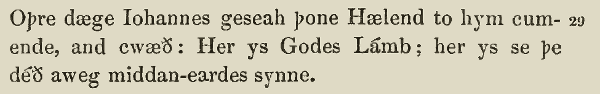
it’s simple to illustrate with language – for example, the change we see in the linguistic trajectory towards present-day English in a verse from John’s gospel:
John 1:29,
West Saxon Gospels, c. 990.
Anothir day Joon say Jhesu comynge to hym, and he seide, Lo! the lomb of God; lo! he that doith awei the synnes of the world. ( Wycliffe Bible, 1395)
The nexte daye Iohn sawe Iesus commyge vnto him and sayde: beholde the lambe of God which taketh awaye the synne of the worlde. ( Tyndale New Testament, 1525)
The next day Iohn seeth Iesus coming vnto him, and saith, Behold the Lambe of God, which taketh away the sinne of the world. ( KJV, 1611)
The next day John seeth Jesus coming unto him, and saith, Behold the Lamb of God, which taketh away the sin of the world. ( KJV, Cambridge Edition)
The next day John saw Jesus coming toward him and said, “Look, the Lamb of God, who takes away the sin of the world!” ( NIV, 2011)
Note well that these “forms”, as we see them here, themselves have many gradations between them, of course. These selections are useful for our illustrative purposes, however. Note that the overall shift to the “modern” text is the cumulative result of many individual changes. To return to our analogy, if every word is a gene, we see shifts in alleles over time as follows:
cwæð → seide → sayde → saith → said
synne → synnes → synne → sinne → sin
to hym cumende → comynge to hym → commyge vnto him → coming vnto him → coming unto him
Though the changes in each word contribute to the overall transformation, each word has only a relatively minor effect on its own. Yet the combined actions of changes in many words, over time, can change West Saxon to modern English. There are not, however, large jumps at any point along the way – each generation of speakers could easily understand their parents and their children – but over time, the shifts are large enough that West Saxon and present-day English are not even close to being the same language.
Next, we’ll consider how changes in alleles can lead to new species – much like change over time can lead to new languages.
Good Butter and Good Cheese – Language, Populations and Speciation
Previously, we drew an extended analogy between genetic change within a population over time, and change within a language over time. While no analogy is perfect, this one is remarkably good – and it will continue to be useful as we now turn to discussing how new species form.

With a last name like Venema, it will come as no surprise to many that I have Frisian ancestors.
Friesland is a province of the Netherlands with a distinct language,
West Frisian, that is one of the most closely-related modern languages to English. My paternal grandparents, immigrants to Canada in the post-World War II era, spoke a delightful hodge-podge of English, Dutch and Frisian to each other, often using mostly Frisian and only reverting to Dutch or English if it happened to have a better word for the concept at hand. As a child, I remember hearing Frisian and noting how similar many of its words were to their English equivalents – far too many similarities, I thought, to be merely coincidence.Some languages retain remarkable similarities, more than could be mere coincidence. The language, West Frisian, comes from Friesland, a province of the Netherlands, and is one of the most closely-related modern languages to English. A well-known sentence will serve as an illustration: it is pronounced
essentially the same in both Frisian and English:
Butter, bread, and green cheese is good English and good Frise.
Bûter, brea, en griene tsiis is goed Ingelsk en goed Frysk.
Later, I would come to understand theThere is a good reason for these striking similarities – English and West Frisian are modern descendants of an ancient language – they share a common ancestral population of speakers. As we have seen, languages change over time. In the case of English and West Frisian, the original population, which spoke a language ancestral to both modern-day English and modern-day West Frisian, was divided: some remained on the European continent, and others travelled to what is present-day England. Once separated, each sub-group – which at the point of separation spoke the same language – went on to acquire differences over time that were independent of each other. In due time, the changes that accumulated in both groups rendered them mutually unintelligible to each other: they had become separate languages. The precise point at which they became “different languages” of course is impossible to pin down, since there was no such precise point when it occurred. Both groups changed their language over time incrementally, as a process on a gradient.
Species form through a process much like language development. Should two populations of the same species become separated, they too can accumulate genetic changes that shift their average characteristics over time – changes that are not shared and averaged across the two groups due to their genetic isolation. In many cases, geographic isolation acts as the first genetic barrier – much like the ancestors of the English parting ways with their continental cousins. Once separated, should enough genetic changes accrue between the two populations, eventually they will not recognize each other as members of the same species – which would be analogous to my experience as a modern English speaker in present-day Friesland.
Species, like languages “begin” as populations – and “begin” isn’t the right word
Our language analogy also helps to counter some common misconceptions about how species form. Often when I am speaking about human origins, folks who have heard about modern humans descending from around 10,000 ancestors wonder how on earth those 10,000People who hear about modern humans descending from a large population wonder how on earth those people suddenly appeared on the scene without ancestors. Of course, they didn’t suddenly appear – they too have a population that gave rise to them, and so on – stretching back to our shared ancestral populations with other apes and beyond. There is in fact no point in our evolutionary history over the last 18 million years or more where our lineage was reduced below 10,000 individuals – and 18 million years ago our lineage was not even close to “human” in any sense, since this time
predates any hominin (i.e. species more closely related to us than to chimpanzees) in the fossil record. The 10,000 number is simply the smallest population size we have in our history over the last several million years. The lineage leading to modern humans experienced what is known as a population bottleneck, a time when our ancestral population size was reduced to around 10,000 breeding individuals, only to expand again afterwards.As far as anyone can tell, the genetic data in fact rules out a single couple for at least half a million years. At 500,000 years ago, our ancestors were not even modern Homo sapiens. A straightforward interpretation of the genetics data is that our ancestors were part of a population in the thousands as far back as we can see.
Despite these explanationsfindings, it is a common misperception to think that species, should one go back far enough, started off with one ancestral breeding pair “becoming different”. Hopefully our language analogy is useful here. It is of course not reasonable to expect that English or West Frisian got its start when two individuals began speaking a new language. The lineage that led to either modern language did so as a population of speakers – and each generation within both lineages was perfectly intelligible to their parents and their offspring. In the same way, species form as populations shift their average characteristics over time – but always remaining the “same species” as their parents and their offspring. So, to speak of a language or a species “beginning” is to hit up against the limits of language. Neither “begins” in some sort of discontinuous sense – they become, over time, in continuity with what came before.
So, one of the reasons for the common expectation that humans had a discontinuous beginning with a single ancestral couple has nothing to do with Genesis or Judeo-Christian theology: I have met many (non-theists who also have this same expectation). We are used to thinking in discontinuous terms – species should have a defined beginning – and we are used to thinking that species therefore begin with a radical change to a single ancestral pair. For evangelical Christians, these incorrect assumptions about how species get their start fit hand in glove with the common view that since species require a discontinuous start, only God can miraculously provide it through an event of special creation. Once one understands how species form as populations over time, however, one is then prepared to investigate the question of how large our population was as we became human – a question we will begin to address in the next post.
Signature in the SNPs
Previously, we drew an extended analogy between how species form and how languages change over time. Through this analogy we came to understand that species, like a group speaking a language, are continuous populations that shift their characteristics incrementally over time. From this analogy we concluded that “species” is a label of convenience for what is in fact a population undergoing continuous, incremental change – just as a “language” is not static but in constant, if gradual, flux. With this understanding we are ready to begin examining our genome with the correct ideas in mind. The question is not, then “when did our species begin?”, since that question is like asking when “English” began. What genetics can address, however, is how many individuals were in our ancestral population as it separated from other species and became a distinct lineage. There are a number of genetic approaches that allow for such estimates, and we will examine a few of them in this series. Importantly, all of the methods return very similar estimates – that our ancestral population has not dropped below about 10,000 individuals over the last several million years.. The most straightforward interpretation of the data is that our ancestral population numbered in the thousands for at least the last 500,000 years. Since the earliest-known anatomically modern humans are present in the fossil record at 200,000 years ago, this minimum population size spans the time during which we biologically “became human” as a population. For a recent detailed description, see
What Genetics Say About Adam and Eve by Steve Schaffner.
Genetic variation and population size
Each of the population-size methods we will examine base their calculations on the amount of genetic variation in present-day human populations. For any given section of DNA in our genome, any one person can have at most only two versions of it – one received from their mother, and the other from their father. A large population, however, can have many more versions than just two. The amount of genetic variation in a population then, is connected to the number of individuals in that population. At its most basic, every estimate of ancestral human population size uses present-day genetic variation to estimate how many ancestors are needed to transmit the observed level of variation to the present day. A large amount of present-day genetic variation requires more ancestors than does a small amount.
The advent of genome sequencing, as you might expect, has shed a great deal of light on how much genetic variation is present in modern human populations. One significant source of human genetic variation comes in the form of what are known as single nucleotide polymorphisms, or “SNPs” (pronounced “snips”). “Polymorphism” simply means “having many forms”. SNPs are single DNA letters that are variable among humans, and we have around 300,000 common SNPs in our genome of 3 billion DNA letters. In other words, the majority of our genomes are identical to each other, but a small number of DNA letter positions on our chromosomes are variable. Consider a short section of DNA sequence for six different individuals, with three variable positions:
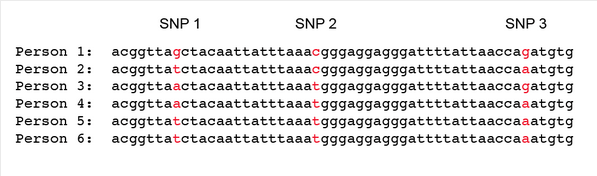
For any one SNP position, there are a maximum of four possible versions (since there are four DNA letters). Once we consider a few SNPs linked together on the same chromosome, however, the number of possible combinations becomes very large. For example, for just the three SNPs shown above, there are 64 different possible combinations (4 x 4 x 4, or 43). Twenty SNPs, on the other hand, would have 420 possible combinations, more than the number of people on the planet. For the six individuals above, we can see that there are five different combinations present. The most likely explanation for these five variants is that they were inherited from five different ancestors, and that persons 5 and 6 inherited their identical combination from the same ancestor. There are other, less likely possibilities, however: some of the combinations might result from new mutations, or from mixing and matching between the different SNPs. For example, person 4 and persons 5 and 6 differ by only one letter: person 4 has an “a” for SNP 1 where persons 5 and 6 have a “t”. One possibility that we need to account for is that person 4 might be descended from the same ancestor as persons 5 and 6, but that a new mutation from t → a occurred at the SNP 1 location. Another possibility is that there was recombination, through a process called “crossing over”, that placed a “t” into this position in person 4. So, when using SNP variation to count the number of likely ancestors, we need to factor in mutation and recombination rates, both of which we can measure directly in humans. In practice, the effects of mutation are small on using SNPs to estimate ancestral population sizes, since the mutation rate in humans is very, very low. Direct measurements of the rate have been done by sequencing the entire genomes of parents and offspring, and on average there are only about 100 – 150 new mutations every time we copy our genome of three billion DNA letters. The effects of recombination can also be minimized by choosing SNPs that are linked closely together on the same chromosome. SNPs that are closely linked together recombine only rarely, since there is so little space for crossing over to occur between them. While scientists factor in mutation and recombination rates, in practice they are not a major issue for SNP-based methods.
In practice, population size estimates based on SNP variation is simply a matter of sequencing a large number of people from around the globe, cataloging them for various SNPs, and estimating how many ancestors they would need to have the SNP variation we see in the present day. As you might expect, different people groups have characteristic sets of SNP variants within them. This makes sense, of course, because we know that the various groups are more closely related to each other than across groups. Tallying up the number of ancestors using this method consistently returns a total minimum population size of about 10,000 individuals: approximately 8,000 ancestors are needed to explain SNP diversity in sub-Saharan Africa, and about 2,000 ancestors for everyone else. SNP diversity in humans is far too large to result from one ancestral couple at any time in the last 200,000 years – we descend from a population. These values are also in good agreement with older, cruder methods of estimating population size from other types of genetic variation, giving us increased confidence that they are reasonable.
Linguistics and the Question of Common Ancestry
Previously, we discussed a method for estimating human ancestral population sizes over the span of our geological history. Anatomically modern humans first appear in the fossil record at about 200,000 years ago, and the SNP-based methods we examined covered a similar time span. These studies, as we saw, indicate that we descend from a population that maintained a minimum of about 10,000 individuals from this point in our history through to the present day. This result, however, often causes confusion about the source of these 10,000 ancestors. As we have discussed, we are used to erroneously thinking in discontinuous terms where species have a sudden start – and as such, it’s common for folks to wonder where these 10,000 people suddenly appeared from.
Think back to our analogy to language evolution, and the origins of the present-day English language. Though we can trace the historical path of English back to the Anglo Saxons at around 900 A.D., we understand that this linguistic group did not suddenly appear on the landscape. Rather, the Anglo Saxons were the descendants of an earlier group—with incremental change, generation by generation—that we traced to a common ancestral population with the speakers of present-day West Frisian that lived at around 400 A.D. on the European continent. Pushing further back in time, one could trace the linguistic history of this group and chart its connections to other related languages.
Human evolution can be understood in much the same way. The minimum population size of 10,000 ancestors did not suddenly appear out of nowhere—they too had an ancestral population that produced them, and so on, deep into the past. Just as “English” slowly emerged over tens of generations, so too our lineage slowly came to be biologically human – over thousands (or tens, or hundreds, of thousands) of generations.
Genomes as linguistic histories
In previous posts in this series, we have examined two lines of evidence for language change over time. The first was change within a language lineage, illustrated with translations of John 1:29 from the time of the Anglo Saxons to the present day. The second line of evidence was to compare distinct modern languages with each other, as we illustrated with two sentences pronounced the same in West Frisian and Modern English:
English: Butter, bread, and green cheese is good English and good Frise.
West Frisian: Bûter, brea, en griene tsiis is goed Ingelsk en goed Frysk.
The reason for these lines of evidence is straightforward: as languages are handed down over time, they accumulate changes. Within a lineage, then, we expect to see evidence of shifts over generations. The same process, however, also would be expected to produce new languages if a common population were separated into two isolated groups.
For biological evolution, then, we would expect equivalent lines of evidence – evidence of change within a specific lineage leading to a present-day species, and evidence that lineages may have split over time to produce new species. For languages, we naturally look to texts; for species, we can look to genomes. Interestingly, genomes have certain features that make these investigations even easier to perform than with languages.
For a language, meaning is required for transmission to the next generation: nonsensical text will be eliminated. Genomes, on the other hand, are quite adept at transmitting nonsensical text. Genomes are copied by DNA-replicating enzymes that are not “aware” of the “meaning” of the DNA sequence they are copying. “Meaning” in this context is biological function, something that the DNA copying enzymes do not have the ability to determine. Whereas a human scribe may fix a misspelled word in a copied manuscript, DNA “scribes” cannot see the intended meaning and fix a previous copying error. As such, DNA mutations (copying errors), once introduced into a population, may be inherited by others – and, given enough time, become the only version of a given sequence in a population. One example of this in the human genome is a DNA copying error we all share – mutations that destroy the function of the enzyme used to make vitamin C. All humans lack this enzyme, called L-gulonolactone oxidase (abbreviated GULO). Though all of us lack this enzyme function, we also all retain much of its DNA sequence in our genomes. Our enzymes keep on transmitting this defective sequence as faithfully as they can, unaware that the enzyme no longer works (and that we must consume a diet rich in vitamin C in order to compensate). As such, our genomes tell us of a time when our lineage was able to synthesize our own vitamin C as other mammals do, and illustrate that our lineage has changed over time.
The second line of evidence we expect from biological evolution is that a lineage may separate, and the two populations go on to form distinct – but closely related – species. The evidence, as we have seen from our analogy using modern West Frisan and modern English, is shared similarities between the two resulting groups. For species, similarities between genomes can be evaluated to look for evidence of shared ancestry. To return to the GULO example, it has long been known that in addition to humans, other primates also lack the ability to synthesize their own vitamin C. DNA sequencing of other primate genomes reveals that they too have the remains of the GULO enzyme sequence, as we do. Further comparison reveals that many of the mutations that remove the function of this enzyme in humans are shared with other primates. One example is a single DNA-letter deletion that removes the function of the gene (highlighted in yellow):
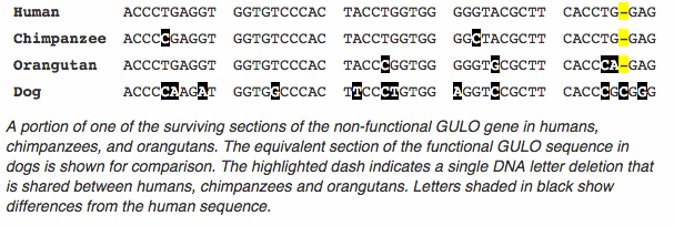
When faced with evidence such as this, there are two competing hypotheses that biologists consider. The first hypothesis is that this shared similarity (a deletion that removes the function of a gene) occurred in the common ancestral population of present-day humans, chimpanzees, and orangutans before this population separated into lineages that led to the present-day species. The alternate, less likely hypothesis, is that this precise mutation occurred three times in three separate lineages. While less likely, this option remains a possibility, and one that a geneticist would take seriously. What is needed, of course, is more evidence from other regions of the genome – while any one shared similarity might be attributed to chance, the combined force of many such similarities would provide a compelling case.
Next, we’ll examine a larger data set to see if the hypothesis of shared ancestry remains supported, and begin to explore how shared ancestry can inform us about our population dynamics as we became human.
Common Ancestry, Nested Hierarchies, and Parsimony
Previously, we introduced the concept of mutations that are shared between species as one line of evidence for common ancestry. In the example we examined, we saw how the deletion of the same DNA letter was present in three primate species: humans, chimpanzees, and orangutans. If indeed these three species share a common ancestral population, then this pattern is easily explained – the mutation occurred in their shared ancestral population, became more common within that population over time, eventually became the only version of that gene in the population, and then was subsequently inherited by the branching populations that went on to become present-day humans, chimpanzees and orangutans. The alternative hypothesis, that humans, chimpanzees, and orangutans do not share a common ancestral population, requires that this precise mutation occurred three times in three separate populations, and replaced the functional version of the gene three times over in those three populations. While such a possibility is rare, for a single gene such a series of improbable events might occur three times independently. In the absence of any other data, a geneticist would rightly hesitate somewhat; though highly suggestive of shared ancestry, such a data set would be too small to draw a firm conclusion.
Of course, in this era of genome sequencing, we now have complete DNA sequences for humans and other great apes to compare to one another. One finding that may be a surprise to non-biologists is that genomes change much, much more slowly than languages do. As we have seen, a mere 1600 years is enough to bring about modern English and Frisian from a common ancestral language – languages that, for all their similarities, are mutually unintelligible to each other despite a relatively recent separation. The human and chimpanzee genomes, on the other hand, are nearly identical to each other. If you restrict the comparison to the small fraction of the genome that contains gene sequences, the two species are over 99% identical to each other. If you expand the analysis to include all sequences (even ones that do not appear to have a sequence-specific function, or repetitive DNA that seems to accumulate in genomes over time), the number hardly shifts, dropping to about 95% identical. To put that in perspective, the human and chimpanzee genomes are more identical to each other than many alternative readings of certain passages in the New Testament, as minor as many of those differences are. And just as no one doubts that two New Testament fragments 95% identical to each other are in fact related through a process of (imperfect) copying, so too it is a significant stretch to argue that the human genome is not related to the chimpanzee genome, given such a high level of shared identity between them. On the whole, our genome and the chimpanzee genome have the features one would predict for slightly modified descendants of a common ancestral genome.
The nose knows (or at least it once did)
Having the complete genome sequences for a variety of great apes makes looking for additional shared mutations a trivial exercise, and it is no exaggeration to say that there are thousands of examples that could be used. One study examining shared mutations in great apes focused on a class of genes used for the sense of smell, known as olfactory receptor genes. The proteins encoded by these genes are present on the cells of the nasal epithelium—the surface of our noses—where they bind to molecules in the air. This binding sends nerve impulses to our brains, which, in specific combinations, we perceive as smells. Primates, as it turns out, have lost a number of genes in this category—and as we saw for the GULO enzyme, we share identical mutations in some of these genes with other primates. For example, in the data set from this study, twelve identical mutations were found to be shared between primates in a particular pattern (shown in red in the diagram below).
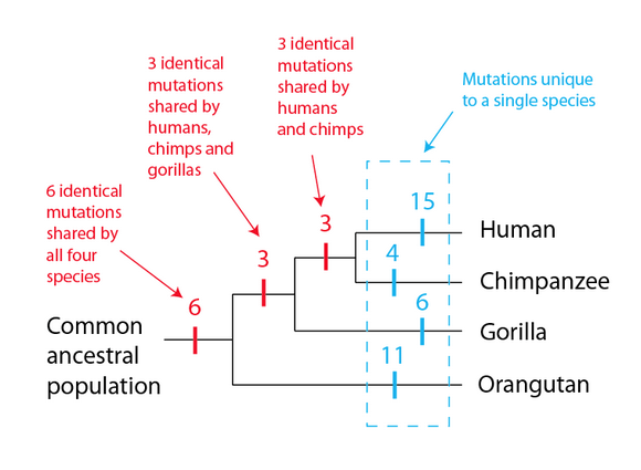
Three of these mutations are shared between humans and chimpanzees only; a further three are shared between humans, chimpanzees and gorillas; and a further six identical mutations are shared between humans, chimpanzees, gorillas and orangutans. This pattern is readily explained by the following: the common ancestral population of all four species has six mutations that occurred prior to the lineage leading to orangutans branched off; three more that occurred before the lineage leading to gorillas branched off; and another three that occurred before the lineages leading to humans and chimpanzees separated. In this model, there are no repeated identical mutation events in separate lineages—every mutation happens only once. Note also what we do not observe—shared mutations that are not part of this pattern. While the researchers found other mutated olfactory genes, none of these mutations were shared, but rather present in only one species. Put another way, in this data set if we see a mutation shared between humans and gorillas, we see those exact mutations in chimpanzees without fail. Likewise, if we see a mutation shared between humans and orangutans, we see those exact mutations in gorillas and chimpanzees, again without fail. The shared mutations make a precise pattern that is exactly the pattern we expect if indeed these species share common ancestral populations that progressively divided into four lineages—a pattern known as a nested hierarchy.
Consider the alternative hypothesis for this data set—that humans, chimpanzees, gorillas, and orangutans do not share common ancestral populations. In order to explain the above data, we would have to postulate a long list of improbable events:
- Six identical mutations occur independently in all four species, and each mutation replaces the functional version of the gene in each species.
- Three identical mutations occur independently in gorillas, chimpanzees, and humans, but not in orangutans. Each mutation replaces the functional version of the gene in the three affected species.
- Three identical mutations occur independently in chimpanzees and humans, but not in gorillas or orangutans. Each mutation replaces the functional version of the gene in both species.
As you can see, the alternative explanation requires numerous, identical mutation events in unrelated species that just happen to match one specific pattern out of thousands of possible patterns – the one pattern predicted by shared ancestry. And once you consider the thousands of shared mutations that conform to this pattern across the great apes, it becomes apparent just how strong the evidence for common ancestry is, and how strained the alternatives are. In scientific terms, common ancestry is a much simpler explanation, requiring far fewer events, and producing the observed pattern as a consequence of the mechanism rather than by chance. In other words, common ancestry is a vastly more satisfactory explanation for what we observe in nature than the alternative hypothesis that humans do not share ancestors with other apes.
As an aside, a third hypothesis is that the pattern of shared mutations is in fact the result of common design, rather than common descent. This option is one that I am often asked aboutis a common question. This hypothesis, however, is even more strained than postulating independent mutation events. In this case, we would have to postulate that, for reasons unknown to us, a designer placed these sequences into these four species with their mutations already in place, and thus not able to function as olfactory receptors. Additionally, the sequences were placed in precisely the pattern that common ancestry would produce. (Alternatively, the designer may have placed functional sequences into these four species but then chose to inactivate them in a specific pattern consistent with common ancestry). While such a possibility cannot be absolutely ruled out, it is very much an ad hoc explanation. After all, we know what these genes are for (contributing to the sense of smell), and we know from the mutations that they carry that they cannot perform that function. Similarly, we know that the GULO enzyme is for making vitamin C, and we know that it is non-functional in primates. The idea that God placed these mutations (and thousands of other examples) into these species in a pattern matching what common ancestry would produce – when in fact common ancestry is false – is something that I findis theologically problematic.
Common ancestry, then, is by far and away the most parsimonious explanation for the data we see. And as I sometimes comment to my students, it’sIt’s possible to view common descent as God’s ordained mechanism for bringing about new species. In this sense, descent is the design.
Variation, populations, and speciation
What then, does this have to do with the central question of this series? The first consideration is that if humans indeed are the product of evolution and share ancestors with other species, we would expect that the process was mediated through populations, since evolution is a population-level phenomenon. Beyond this, however, is a way to use related species to estimate population size during the speciation process. In the above examples, each mutation completely replaced the functional version of the gene in the population before the lineages separated. In some cases, however, we would expect lineages to separate with genetic variation present for a given gene – i.e. with two or more alleles present in the population when it is separated into two lineages. Once we have a clear picture of how species are related to each other, we can search for genes that happened to have two or more variants during a speciation event, and use such genes to estimate population sizes for the resulting species – a topic we will explore next.
You Say To-may-to, I Say To-mah-to
Throughout this article, we have discussed how evolution is a population-level phenomenon, where average characteristics shift incrementally over time. As we have seen, new DNA variants that arise from mutation events are the physical basis for this process. These mutations occur in one individual and then may spread to become more common in a population – perhaps even completely replacing all other variants of that sequence within a population. Just as a language may slowly change to a new spelling of a word, so too a population may shift from one DNA variant to another over time.
In this process, however, populations may maintain two (or more) variants for a long period of time. Again, language change over time is a useful analogy here. If we consider modern English as an example, there exist some variant spellings that are currently seen as “correct” within their local setting. Where an American would use forms such as “harbor” or “neighbor”, those from the United Kingdom, Canadians and others would use slightly different spellings: “harbour” and “neighbour” (and even as I write this, my American-made word processor balks at those versions). For modern English as a whole, then, we maintain some acceptable variation in spelling for certain words – we have not yet universally “decided” on one correct spelling for these words, and perhaps we never will.
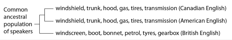
If we were to compare British English, American English, and Canadian English as a whole, Canadian and American English are more similar to each other, because they (in general) share a more recent common population of speakers than either does with British English (due mostly to more extensive mixing between Americans and Canadians since the Americas were colonized). This can easily be demonstrated– Canadians and Americans consistently use words and phrases that are more alike than either is to British English. As any American or Canadian home mechanic will tell you, reading a British automotive repair manual can be an exercise in confusion. Whereas Canadians and Americans use the same terminology, our cousins across the Atlantic use different terms for many car parts:
Other examples are easily found: no one in Canada says “aluminium” as British speakers do, opting rather for the American form “aluminum”. One of myA favorite (favourite?) examples comes from N.T. Wright: if you hear someone say “I’m mad about my flat” it makes all the difference in the world if they are North American or British. For those of us in North America, it means we’re upset about a tire puncture – for Brits, it means one is enthusiastic about one’s living arrangements. American and Canadian English consistently group together, since they are closer relatives to each other than either is to British English. In biological terms, Canadians and Americans share a more recent common ancestral population.
Yet, as any Canadian knows, despite our near-complete affinity with American English, there are few spellings that buck the overall trend. The –our vs. –or forms are a good example:
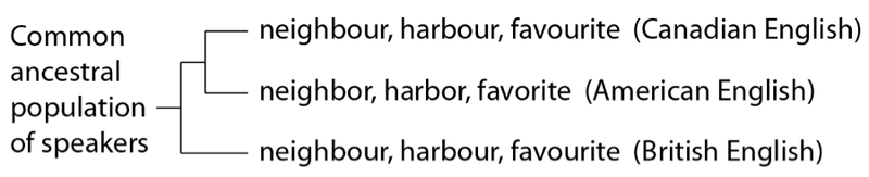
In this case, we see closer affinity between Canadian and British English – even though, on the whole, Canadian and American English are closer relatives. How is this possible? The answer is straightforward – although most of Canadian and American English shares a more recent common source than either does with British English, some Canadian words share a more recent common source with British words.
In the case of the “-or” vs. “-our” spellings, these were acceptably variable in the United Kingdom prior to the colonization of North America: while both forms were used, it seems that the “-or” versions were less common. When English speakers colonized North America, they brought both forms along for the ride. Examples of “-our” spellings can be found in early American texts. For example, honour makes an appearance in an early draft of the Declaration of Independence, though the final form has honor. In general, in the United States, the “-our” forms were lost, and in Canada, the “-or” forms were lost. We can represent these events on a phylogeny leading to the present-day forms, as if these languages were species, and the words within them were DNA variation:
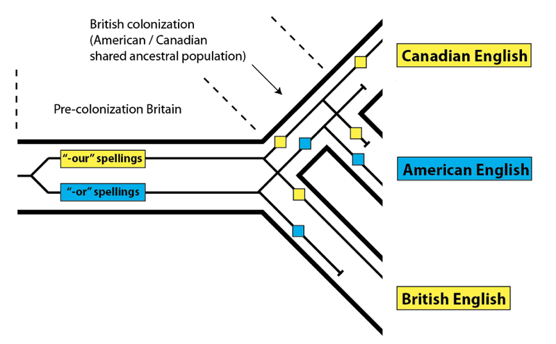
As we can see, this process resulted in Canadian and British English matching more closely to the exclusion of American English for these specific word spellings, even though, as a whole, American and Canadian English are closer relatives. The reason for the pattern is simple – not every variant spelling from the original ancestral population (pre-colonization Britain) sorted down to every descendant population.
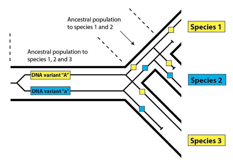
This effect is called incomplete lineage sorting, and it works in exactly the same way in biological populations as it does in linguistic ones. Instead of variant spellings, DNA variants present within an ancestral population may not sort completely down to every descendant species due to losses along the way:

Here, as before, we see that the variants present in Species 1 and 3 match more closely than either does with Species 2, even though Species 1 and 2 share a more recent common ancestral population. In order to find such DNA variants that buck the overall relatedness trend, we need to be confident that we have determined the true pattern of relatedness for the species we are examining. In practice, this is not difficult – we simply look at the overall pattern of relatedness between species at the DNA level. Species 1 and 2 in the diagram above will share DNA similarities to the exclusion of Species 3 most of the time in a nested hierarchy. The overall pattern will be consistent, but a few variants will produce a pattern that does not match the species pattern – a pattern said to be discordant with the pattern of overall species relatedness. As we have seen with languages, these discordant variants are useful for investigating the features of the populations that gave rise to them. Look again at the species diagram above. The fact that we see incomplete lineage sorting for DNA variants “A” and “a” tells us (1) that both variants were present in the common ancestral population of all three species, and (2) that both variants were present in the common ancestral population of Species 1 and 2. Knowing that these populations had these variants present within them allows us to estimate their level of DNA variation generally, which in turn allows us to estimate their population size.
Next, we will apply this technique to the genomes of humans, chimpanzees, and gorillas – and discuss how it sheds light on the population size of our lineage as we separated from other great apes on the long road to becoming human.
Coalescence, Incomplete Lineage Sorting, and Great Ape Ancestral Population Sizes
In the last post in this series, we introduced the concept of incomplete lineage sorting using the distribution of words with alternative spellings in Canadian English, American English, and British English. As we saw, the variation in spelling words with “-our” and “-or” was present in the common ancestral population of all three groups. Despite sharing a more recent common ancestral population with Americans in general, Canadians use the “-our”spellings along with their British cousins in contrast to the American “-or” versions:

This type of pattern, as we noted, is also found in the DNA of related organisms that separate from each other over a relatively short timescale (in this context, within a few million years). Since the lineages leading to humans and other great apes went their separate ways within the last few million years, we expect that this pattern should apply to a portion of the human genome. While we should match our closest relative (chimpanzee) most often, we also expect that the human genome will match the gorilla genome more closely for some of our DNA sequences:
The reason that we expect to match with chimpanzees most often is straightforward: we shared a common ancestral population with them for a longer period than we did with gorillas, which branched off earlier. We do, however, expect to match with gorillas a portion of the time – just as Canadians and Brits match on occasion despite Canadians sharing a longer common history with Americans. And as we saw for alternative spellings, a discordant DNA pattern – one that bucks the overall trend – lets us know that the DNA variants in question were both present in the common ancestral population of all three species (in this case, humans, chimpanzees, and gorillas) as well as in the common ancestral population of the two most closely-related species (in this case, humans and chimpanzees).
One difference between words and DNA sequences is that while an individual might be inconsistent with their spelling – such as a Canadian using American forms when writing for a predominantly American audience – it is not possible for an organism to be inconsistent with the DNA variants they possess. Humans, like all other mammals, have two copies of their DNA sequences – one they inherit from their mothers, the other from their fathers. As such, if we can measure how much DNA variation a population had, we can estimate its population size. More importantly in this case, if we can measure the proportion of DNA sequences in the discordant pattern for three species, we can use that information to infer the ancestral population size of the two more closely related species.
Coalescent theory 101
Note: unfortunately, there is no easy way to explain how this is done without delving a bit into the theory and math behind it. If this gets too complicated, feel free to skip this section and scroll down to the “doing the math” section below.
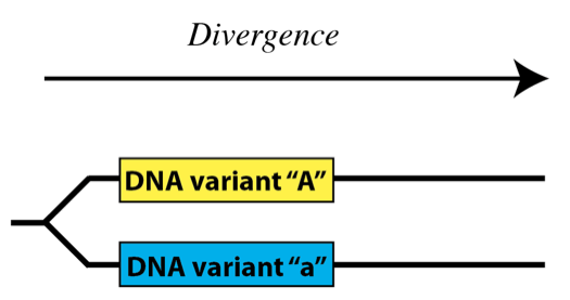
One way to think about DNA variation in populations is to think of it as time goes forward. In this case, DNA variants arise through mutation and diverge from one another within a population:
Another, equally valid way to think about it is to imagine time going backward – in this case, variant DNA sequences become the same, or coalesce as we go back in time:
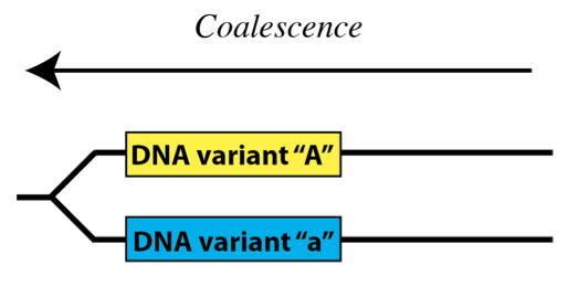
The probability of any two sequences coalescing as we move back in time is the probability that they share the same ancestral sequence – that they are descended from the same original sequence. The probability that they are the descendent of any randomly-chosen ancestral sequence depends on the number of sequences present in the population – in other words, the size of the population.
Let’s return to the example we looked at before:

In this case, reading from right to left (i.e. travelling back in time) we would say that the human and gorilla variants (in yellow) we see in the present day coalesce with each other before they coalesce with the blue variant we see in chimpanzees (the yellow one having been lost). If you trace the yellow variants, they connect with each other sooner than either does with the blue variant. Because the yellow and blue variants do not coalesce with one another until we reach the (human, chimpanzee, gorilla) common ancestral population, there are several possible patterns that might result once such a population undergoes speciation into three descendent species. One possible pattern is the one in the diagram: the human and gorilla sequences coalesce first, followed by coalescence with chimpanzee (what we would call a (HG)C pattern). Another possibility, not shown, would be the gorilla and chimpanzee sequences coalescing first, followed by the human sequence (a (GC)H pattern). The final possibility, also not shown, would be the one that is usually produced – humans and chimpanzees coalesce first, followed by gorilla (the usual (HC)G pattern). Two of the three possible patterns, then, are discordant – (HG)C and (GC)H – and one is not discordant: (HC)G. So, 2/3 of the possibilities produce a discordant pattern, and 1/3 produce the “correct” pattern that matches the overall species pattern.
Notice that one requirement for a discordant pattern to result is that the two DNA variants in the most closely related species (humans and chimpanzees) cannot coalesce in the common ancestral population of those species. The probability that any two sequences will not coalesce in a population over time t is as follows:
In this equation, t = time in years that the common ancestral population in question persists, N = the population size, and g = the generation time in years. (N is multiplied by 2 because every individual carries two DNA sequences.)
From this formula, we can derive the probability that we will see a discordant pattern for any given DNA sequence in three related species. We require that the variants not coalesce, and we have shown that if they do not coalesce, 2 of the 3 outcomes are discordant. So, the probability of observing a discordant pattern is as follows:
Doing the math
With this equation in hand, we are now ready to apply it to what we actually observe in the human, chimpanzee, and gorilla genomes. Using paleontological and genetic data, the time span that humans and chimpanzees shared a common ancestral population after the gorilla lineage branched off is estimated to be 2 million years (t). Using an estimate of generation time of 20 years for all species throughout this process (a value consistent with that observed in present-day great apes) leaves us only with two factors outstanding: the population size of the (human chimpanzee) common ancestral population, and the proportion of DNA sequences we would predict to be in a discordant pattern. Prior to full-genome sequencing of gorillas that allowed for determining the latter, it was predicted, based on genetic evidence, that this population numbered around 50,000 individuals. This value, when plugged into the equation, predicts that 25% of the time we expect a discordant pattern when examining human, chimpanzee, and gorilla sequences. The actual result is about 30%, suggesting a population of about 62,000 individuals. This result adds further support to the prior evidence that the common ancestral population of humans and chimpanzees was large – far larger than even the bottleneck to ~10,000 on the human lineage after the separation from the chimpanzee lineage.
The publication of the complete orangutan genome in 2011 allowed for the same calculations to be made for the (human, chimpanzee, gorilla) ancestral population, since the orangutan lineage branches off the primate tree prior to the (human, chimpanzee, gorilla) speciation events. Once again, predictions were made based on prior population size estimates, and once again the estimates closely matched the observed values – the common ancestral population of (humans, chimpanzees, and gorillas) was of similar size to the (human, chimpanzee) common ancestral population.
Implications for human origins
The conclusions of this article are substatially revised, but BioLogos claimed they were “unchanged”. Moreover, analysis of “incomplete lineage sorting” does not demonstrate the conclusions stated here.
While this quantitative data is not as easy to appreciate as other sorts of evidence we have examined, it nonetheless is compelling: humans, chimpanzees, and gorillas have, within their genomes, the exact pattern of incomplete lineage sorting predicted by (a) relatedness as evidenced by all other lines of genomic evidence (such as shared mutations in individual genes) and (b) large ancestral population sizes throughout the speciation process. The smallest population our lineage was reduced to in the last 15 million years or more, then, was to the bottleneck of 10,000 individuals once our lineage parted ways with the chimpanzee lineage.
In this next article in this series, we’ll expand our discussion to include recent objections by some Christians to these lines of evidence – objections that argue for the credibility of still holding to a recent single pair who are the genetic ancestors of all humans.
References with broken or unresolvable links were removed. Authors and accurate titles were added to resolved references.
References
Loren Haarsma, Why the Church Needs Multiple Theories of Original Sin, BioLogos, 2013.
Tenesa, A., et al (2007). Recent human effective population size estimated from linkage disequilibrium.Genome Res 17 (4) 520-526. https://doi.org/10.1101/gr.6023607
McEvoy, B.P. et al (2011). Human population dispersal “Out of Africa” estimated from linkage disequilibrium and allele frequencies of SNPs. Genome Res 21 (6) 821-829. https://doi.org/10.1101/gr.119636.110
Dennis Venema and Darrel Falk. Signature in the Pseudogenes, BioLogos, 2014.
Gilad, YG., Man, O., Paabo, S., and Lancet, D. 2003. Human specific loss of olfactory receptor genes. Proc. Natl. Acad. Sci. 100: 3324-3327. https://doi.org/10.1073/pnas.0535697100
Hobolth et. al., 2011. Incomplete lineage sorting patterns among human, chimpanzee, and orangutan suggest recent orangutan speciation and widespread selection. Genome Research 21: 349-356. https://doi.org/10.1101/gr.114751.110
S. Joshua Swamidass, Three Stories on Adam, Peaceful Science, 2018. https://doi.org/10.54739/3doe
Deborah Haarsma, Truth Seeking in Science, BioLogos, 2020.
S. Joshua Swamidass, 18 Million Years Ago Means…500,000?, Peaceful Science Forum, 2021.
Apr 10, 2022
Apr 25, 2022
Jul 20, 2026